Wrangling Datasets

Reading, Joining, and Pivoting

Mine Doğucu

Joining Datasets

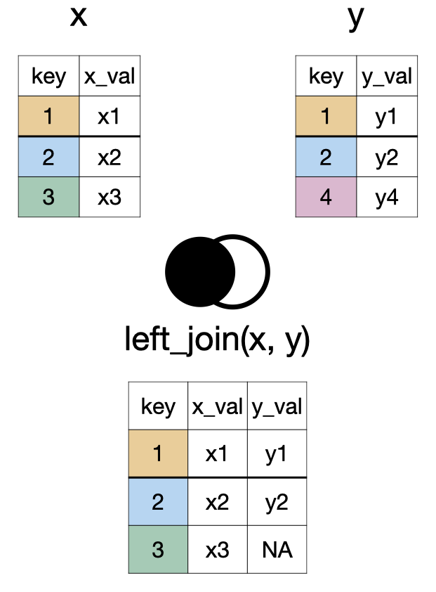
left_join(x, y)

A diagram showing two tables, X and Y, being combined into a new table. Table X has columns 'key' and 'x_val', with keys 1, 2, 3. Table Y has 'key' and 'y_val', with keys 1, 2, 4. The new combined table includes all rows from Table X. For each key present in both tables (1 and 2), the matching 'y_val' from Table Y is added. For keys only in Table X (key 3), the 'y_val' column is filled with 'NA' (Not Applicable)

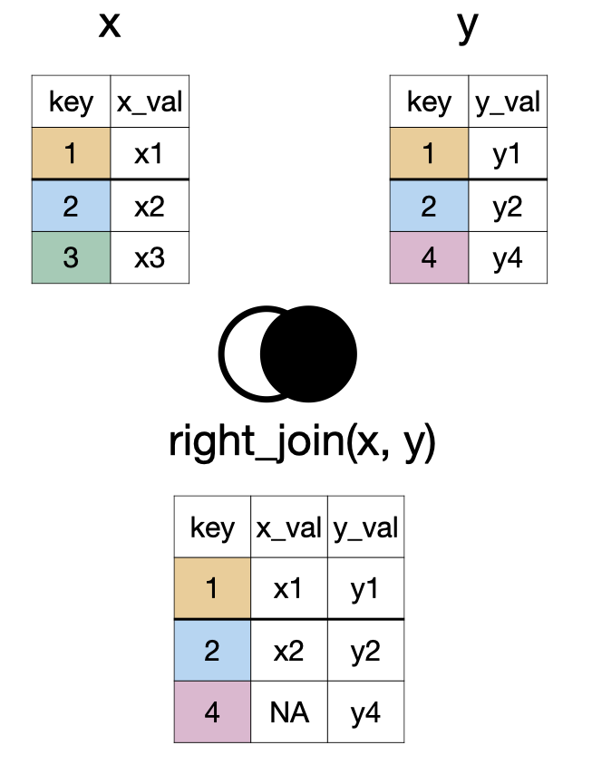
right_join(x, y)

A diagram showing two tables, X and Y, being merged based on a shared 'key' column. Table X has keys 1, 2, 3; Table Y has keys 1, 2, 4. The resulting combined table contains all rows from Table Y. Where keys match in both tables (1 and 2), corresponding values from X are included. For keys only present in Y (key 4), the 'x_val' column shows 'NA' (Not Applicable).

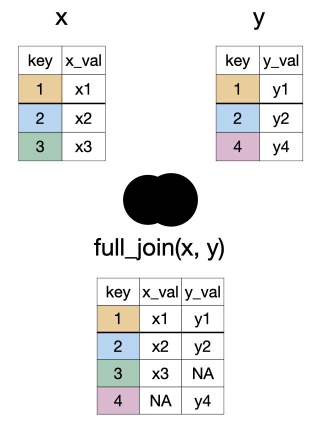
full_join(x, y)

A diagram showing two tables, X and Y, being merged based on a shared 'key' column into a new combined table. Table X has keys 1, 2, 3; Table Y has keys 1, 2, 4. The resulting table includes all keys present in either X or Y (keys 1, 2, 3, 4). For keys found in both tables (1 and 2), corresponding values from both X ('x_val') and Y ('y_val') are shown. For keys only in Table X (key 3), its 'x_val' is included, and 'y_val' is marked 'NA' (Not Applicable). For keys only in Table Y (key 4), its 'y_val' is included, and 'x_val' is marked 'NA'

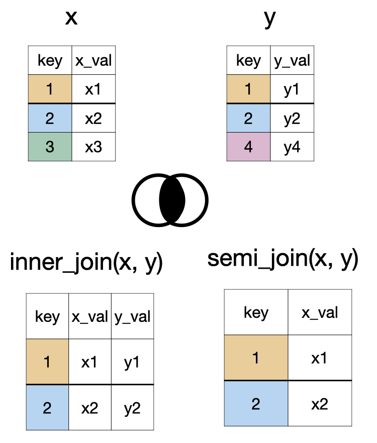
inner_join(x, y) and semi_join(x, y)

A diagram showing two ways to process data from two tables, X and Y, based on a common 'key' column. Table X has keys 1, 2, 3, with an 'x_val' for each. Table Y has keys 1, 2, 4, with a 'y_val' for each. 1.  Inner Combine (labeled 'inner_join'): A new table is created that only includes rows where the 'key' is found in *both* Table X and Table Y (keys 1 and 2). For these matching keys, the new table displays the key, its 'x_val' from Table X, and its 'y_val' from Table Y. 2. Semi Combine (labeled 'semi_join'): A new table is created by taking only those rows from Table X whose 'key' also  appears in Table Y (keys 1 and 2). This new table only displays the 'key' and 'x_val' from Table X.

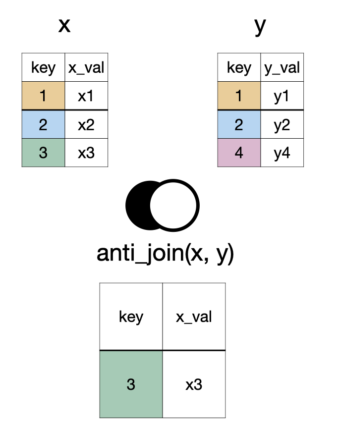
anti_join(x, y)

A diagram showing two tables, X and Y, being processed to create a new table. Table X has keys 1, 2, 3, with corresponding 'x_val' values. Table Y has keys 1, 2, 4, with corresponding 'y_val' values. The new table, labeled 'anti_join(x, y)', is formed by taking only those rows from Table X whose 'key' is *not* found in Table Y. In this example, only the row with key 3 from Table X (and its 'x_val') is included in the final result.

something_join(x, y)

Function x y
Type rows columns rows columns
left_join() all all matched all
right_join() matched all all all
full_join() all all all all
inner_join() matched all matched all
semi_join() matched all none none
anti_join() unmatched all none none

Data

artists
# A tibble: 3 × 2
  name          followers
  <chr>             <dbl>
1 Beyoncé        24757958
2 Taylor Swift   33098116
3 Ariana Grande  51807131
songs
# A tibble: 5 × 4
  name          song_name                            album_name  song_popularity
  <chr>         <chr>                                <chr>                 <dbl>
1 Beyoncé       Savage Remix (feat. Beyoncé)         Savage Rem…              83
2 Taylor Swift  cardigan                             folklore                 85
3 Drake         Laugh Now Cry Later (feat. Lil Durk) Laugh Now …              95
4 Beyoncé       Halo                                 I AM…SASHA…              NA
5 Ariana Grande Stuck with U (with Justin Bieber)    Stuck with…              NA
albums
# A tibble: 4 × 2
  album_name                           album_release_date
  <chr>                                <date>            
1 Savage Remix (feat. Beyoncé)         2020-04-29        
2 I AM…SASHA FIERCE                    2008-11-14        
3 Stuck with U                         2020-05-08        
4 Laugh Now Cry Later (feat. Lil Durk) 2020-08-14        

Relational Schema

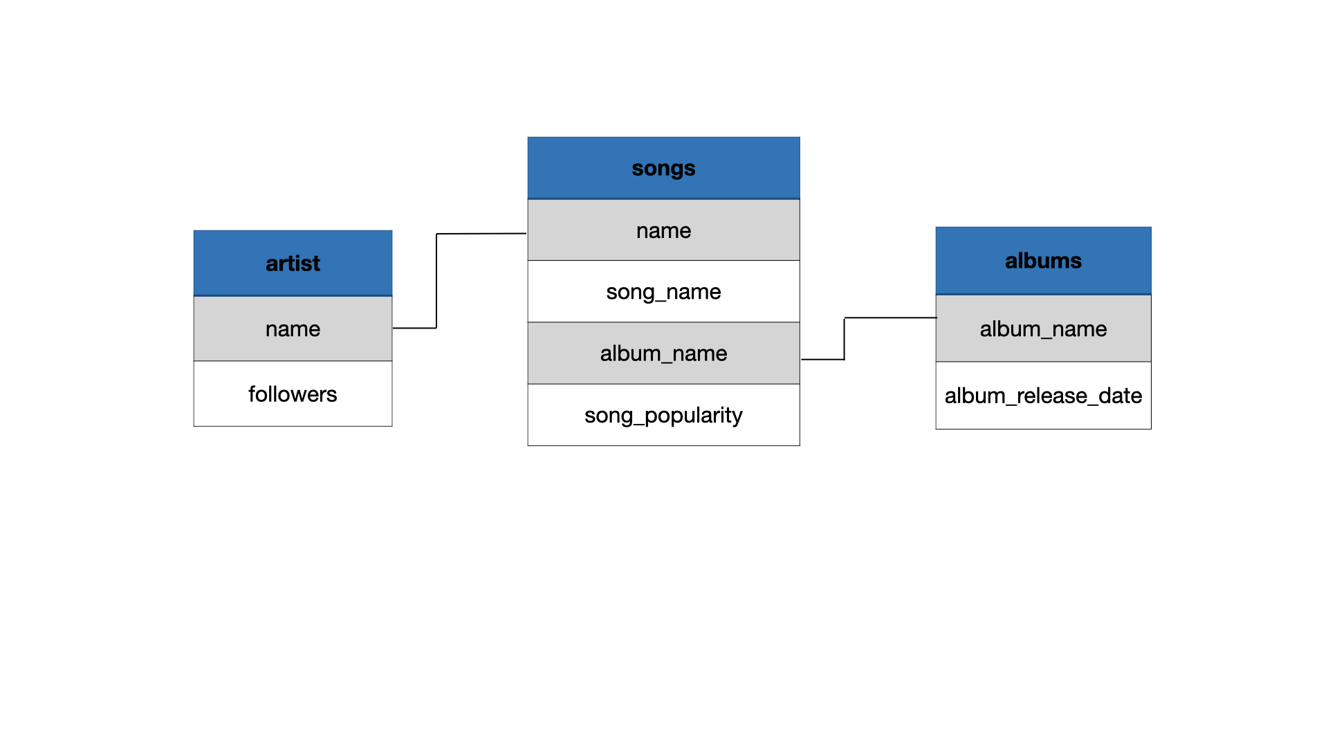
A diagram shows three related collections of music information: 'artist', 'songs', and 'albums'. The 'artist' collection includes the artist's name and their number of followers. The 'songs' collection lists the artist's name, the song's name, the album's name it's on, and its popularity. The 'albums' collection contains the album's name and its release date. Lines connect the artist's name from the 'artist' collection to the artist's name in the 'songs' collection, and similarly, album names link the 'songs' collection to the 'albums' collection. This structure connects song details to their respective artists and albums.

left_join()

left_join(songs, artists)
# A tibble: 5 × 5
  name          song_name                   album_name song_popularity followers
  <chr>         <chr>                       <chr>                <dbl>     <dbl>
1 Beyoncé       Savage Remix (feat. Beyonc… Savage Re…              83  24757958
2 Taylor Swift  cardigan                    folklore                85  33098116
3 Drake         Laugh Now Cry Later (feat.… Laugh Now…              95        NA
4 Beyoncé       Halo                        I AM…SASH…              NA  24757958
5 Ariana Grande Stuck with U (with Justin … Stuck wit…              NA  51807131

right_join()

right_join(songs, artists)
# A tibble: 4 × 5
  name          song_name                   album_name song_popularity followers
  <chr>         <chr>                       <chr>                <dbl>     <dbl>
1 Beyoncé       Savage Remix (feat. Beyonc… Savage Re…              83  24757958
2 Taylor Swift  cardigan                    folklore                85  33098116
3 Beyoncé       Halo                        I AM…SASH…              NA  24757958
4 Ariana Grande Stuck with U (with Justin … Stuck wit…              NA  51807131

full_join()

full_join(songs, artists, by = "name")
# A tibble: 5 × 5
  name          song_name                   album_name song_popularity followers
  <chr>         <chr>                       <chr>                <dbl>     <dbl>
1 Beyoncé       Savage Remix (feat. Beyonc… Savage Re…              83  24757958
2 Taylor Swift  cardigan                    folklore                85  33098116
3 Drake         Laugh Now Cry Later (feat.… Laugh Now…              95        NA
4 Beyoncé       Halo                        I AM…SASH…              NA  24757958
5 Ariana Grande Stuck with U (with Justin … Stuck wit…              NA  51807131

full_join() x2

full_join(songs, artists, by = "name") |> 
  full_join(albums, by = "album_name")
# A tibble: 5 × 6
  name         song_name album_name song_popularity followers album_release_date
  <chr>        <chr>     <chr>                <dbl>     <dbl> <date>            
1 Beyoncé      Savage R… Savage Re…              83  24757958 2020-04-29        
2 Taylor Swift cardigan  folklore                85  33098116 NA                
3 Drake        Laugh No… Laugh Now…              95        NA 2020-08-14        
4 Beyoncé      Halo      I AM…SASH…              NA  24757958 2008-11-14        
5 Ariana Gran… Stuck wi… Stuck wit…              NA  51807131 2020-05-08        

Reading (Importing) Datasets

Importing .csv Data

readr::read_csv("dataset.csv")

Importing Excel Data

readxl::read_excel("dataset.xlsx")

Importing Excel Data

readxl::read_excel("dataset.xlsx", sheet = 2)

Importing SAS, SPSS, Stata Data

library(haven)
# SAS
read_sas("dataset.sas7bdat")
# SPSS
read_sav("dataset.sav")
# Stata
read_dta("dataset.dta")

Where is the dataset file?

Importing data will depend on where the dataset is on your computer. However we use the help of here::here() function. This function sets the working directory to the project folder (i.e. where the .Rproj file is).

read_csv(here::here("data/dataset.csv"))

Pivoting Datasets

Pivoting

In tidyverse (specifically {tidyr}), pivoting refers to reshaping a data frame so that it is either:

longer: more rows, fewer columns, or
wider: fewer rows, more columns.

Data

gapminder is in long format: one row per country-year

library(gapminder)
data(gapminder)
gapminder
# A tibble: 1,704 × 6
   country     continent  year lifeExp      pop gdpPercap
   <fct>       <fct>     <int>   <dbl>    <int>     <dbl>
 1 Afghanistan Asia       1952    28.8  8425333      779.
 2 Afghanistan Asia       1957    30.3  9240934      821.
 3 Afghanistan Asia       1962    32.0 10267083      853.
 4 Afghanistan Asia       1967    34.0 11537966      836.
 5 Afghanistan Asia       1972    36.1 13079460      740.
 6 Afghanistan Asia       1977    38.4 14880372      786.
 7 Afghanistan Asia       1982    39.9 12881816      978.
 8 Afghanistan Asia       1987    40.8 13867957      852.
 9 Afghanistan Asia       1992    41.7 16317921      649.
10 Afghanistan Asia       1997    41.8 22227415      635.
# ℹ 1,694 more rows

pivot_wider(): Long → Wide

life_wide <- gapminder |>
  select(country, year, lifeExp) |>
  pivot_wider(
    names_from = year,
    values_from = lifeExp
  )

life_wide
# A tibble: 142 × 13
   country `1952` `1957` `1962` `1967` `1972` `1977` `1982` `1987` `1992` `1997`
   <fct>    <dbl>  <dbl>  <dbl>  <dbl>  <dbl>  <dbl>  <dbl>  <dbl>  <dbl>  <dbl>
 1 Afghan…   28.8   30.3   32.0   34.0   36.1   38.4   39.9   40.8   41.7   41.8
 2 Albania   55.2   59.3   64.8   66.2   67.7   68.9   70.4   72     71.6   73.0
 3 Algeria   43.1   45.7   48.3   51.4   54.5   58.0   61.4   65.8   67.7   69.2
 4 Angola    30.0   32.0   34     36.0   37.9   39.5   39.9   39.9   40.6   41.0
 5 Argent…   62.5   64.4   65.1   65.6   67.1   68.5   69.9   70.8   71.9   73.3
 6 Austra…   69.1   70.3   70.9   71.1   71.9   73.5   74.7   76.3   77.6   78.8
 7 Austria   66.8   67.5   69.5   70.1   70.6   72.2   73.2   74.9   76.0   77.5
 8 Bahrain   50.9   53.8   56.9   59.9   63.3   65.6   69.1   70.8   72.6   73.9
 9 Bangla…   37.5   39.3   41.2   43.5   45.3   46.9   50.0   52.8   56.0   59.4
10 Belgium   68     69.2   70.2   70.9   71.4   72.8   73.9   75.4   76.5   77.5
# ℹ 132 more rows
# ℹ 2 more variables: `2002` <dbl>, `2007` <dbl>

pivot_wider(): What Happened?

pivot_wider(
  names_from = year,     # column whose VALUES become new column names
  values_from = lifeExp  # column whose VALUES fill the new columns
)
  • Each unique year becomes its own column
  • lifeExp values get spread into those columns
  • One row per country remains

Great for making tables or comparing across time side by side.

pivot_longer(): Wide → Long

Now reverse it — take life_wide back to long format:

life_long <- life_wide |>
  pivot_longer(
    cols = -country,          # all columns except country
    names_to = "year",
    values_to = "lifeExp"
  )

life_long
# A tibble: 1,704 × 3
   country     year  lifeExp
   <fct>       <chr>   <dbl>
 1 Afghanistan 1952     28.8
 2 Afghanistan 1957     30.3
 3 Afghanistan 1962     32.0
 4 Afghanistan 1967     34.0
 5 Afghanistan 1972     36.1
 6 Afghanistan 1977     38.4
 7 Afghanistan 1982     39.9
 8 Afghanistan 1987     40.8
 9 Afghanistan 1992     41.7
10 Afghanistan 1997     41.8
# ℹ 1,694 more rows

pivot_longer(): What Happened?

pivot_longer(
  cols = -country,       # columns to gather (all but country)
  names_to = "year",      # new column to hold old column NAMES
  values_to = "lifeExp"   # new column to hold the VALUES
)
  • Many columns collapse into two: year and lifeExp
  • country is repeated across rows
  • This is the tidy, “one row per observation” shape

Why Go Wide → Long?

life_long |>
  mutate(year = as.numeric(year)) |>
  filter(country %in% c("Canada", "China", "Nigeria")) |>
  ggplot(aes(year, lifeExp, color = country)) +
  geom_line() +
  theme_minimal(base_size = 20)
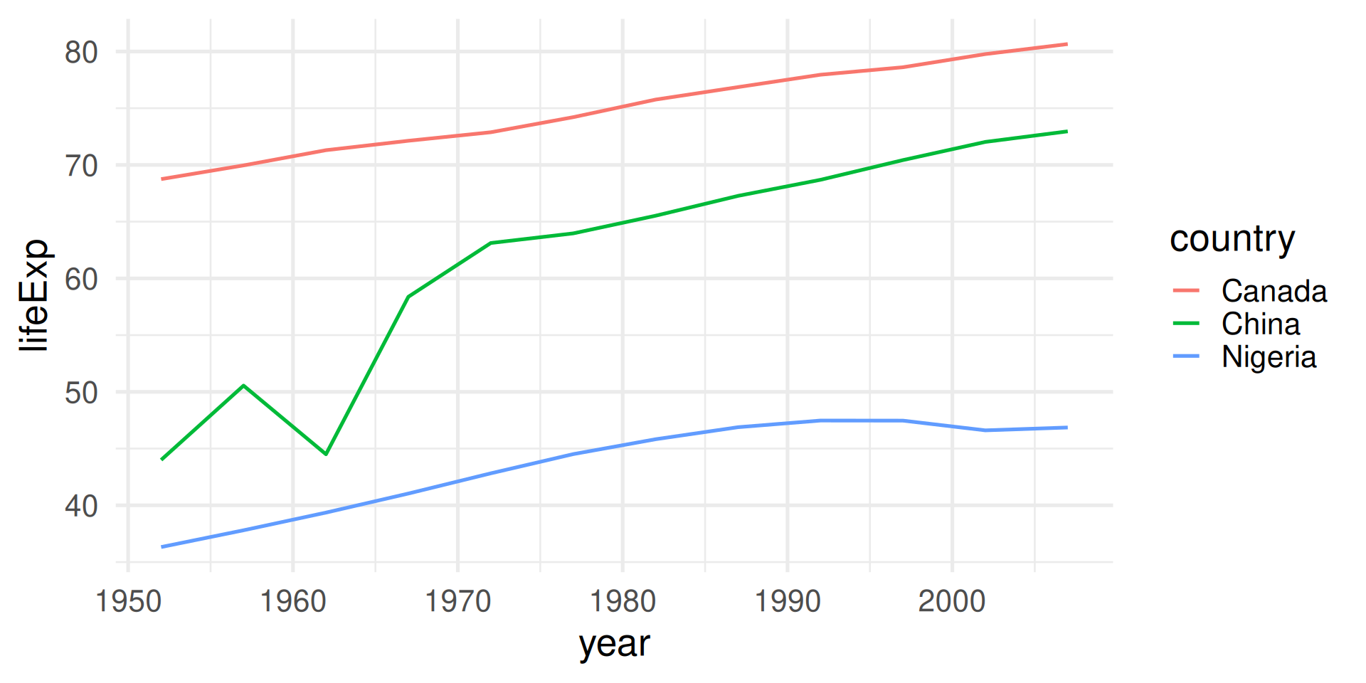
a geom line graph with year on the x axis and life expectancy on the y-axis. The years range from about 1950 to 2010. There are three trajectory lines for three countries Canada, China, and Nigeria.

Why Go Long → Wide?

gapminder |>
  filter(continent == "Oceania") |>
  select(country, year, gdpPercap) |>
  pivot_wider(names_from = country, values_from = gdpPercap)
# A tibble: 12 × 3
    year Australia `New Zealand`
   <int>     <dbl>         <dbl>
 1  1952    10040.        10557.
 2  1957    10950.        12247.
 3  1962    12217.        13176.
 4  1967    14526.        14464.
 5  1972    16789.        16046.
 6  1977    18334.        16234.
 7  1982    19477.        17632.
 8  1987    21889.        19007.
 9  1992    23425.        18363.
10  1997    26998.        21050.
11  2002    30688.        23190.
12  2007    34435.        25185.

Fun side track

The {ggplot2} package has many “extensions” by the tidyverse team and others in the community.

One of these packages is {gganimate} which shows an excellent use of the gapminder data.

If you like thinking about data and public health, you might like Hans Rosling’s talk The best stats you’ve ever seen. You can also take the Gapminder Test.