Some books and some software put the standard deviation (not the variance) as the second number. In R, pnorm(), qnorm(), and rnorm() all use the standard deviation:
pnorm(1200, mean = 1000, sd = 200)
Always check whether the second number is the standard deviation or the variance. Writing it as \(200^2\) makes it clear.
Reading the notation
Exercise
For each normal distribution, find the mean, the variance, and the standard deviation.
\(Y \sim N(10, 4)\)
\(Z \sim N(0, 1)\)
\(W \sim N(-3, 3^2)\)
SAT Math scores have mean 500 and standard deviation 100.
Note: \(N(0, 1)\) in (b) is called the standard normal distribution.
Not just for \(X\)
The random variable on the left of \(\sim\) can be many things.
What can be normally distributed: an observation or a population parameter
Notation
What is normally distributed?
\(X \sim N(1000, 200^2)\)
a random observation (in the population, and so also in a sample): the SAT score of one test taker
\(\mu \sim N(7, 0.5^2)\)
a random population parameter: our belief about the mean hours of sleep of all Harvard students
In a few weeks, we will see that a random sample statistic, like \(\bar{X}\), can also be normally distributed.
This is why we say “mean” and “variance” for the two numbers in \(N(\ , \ )\) rather than giving them their own symbols: sometimes the random variable itself is a mean, like \(\mu\)!
Probability as area
Area = probability
The total area under a normal curve is 1. The probability that the random variable falls in an interval is the area under the curve over that interval.
We will never calculate these areas by hand. We will use functions.
The plot_normal() function
plot_normal(random_variable ="x", # "x", "x_bar", "p", "mu", or "pi"mean =1000, # mean of the normal distributionsd =200, # standard deviation (or variance = 40000)lower =800, # shade from here...upper =1400) # ...to here
It draws the normal curve with the random variable on the x-axis.
It shades the area between lower and upper and writes the area under the plot.
Leave out lower to shade everything below upper, and leave out upper to shade everything above lower.
The calc_prob_normal() function
plot_normal() draws the picture. To get the probability as a number that you can use in your answers, use calc_prob_normal() with the same arguments:
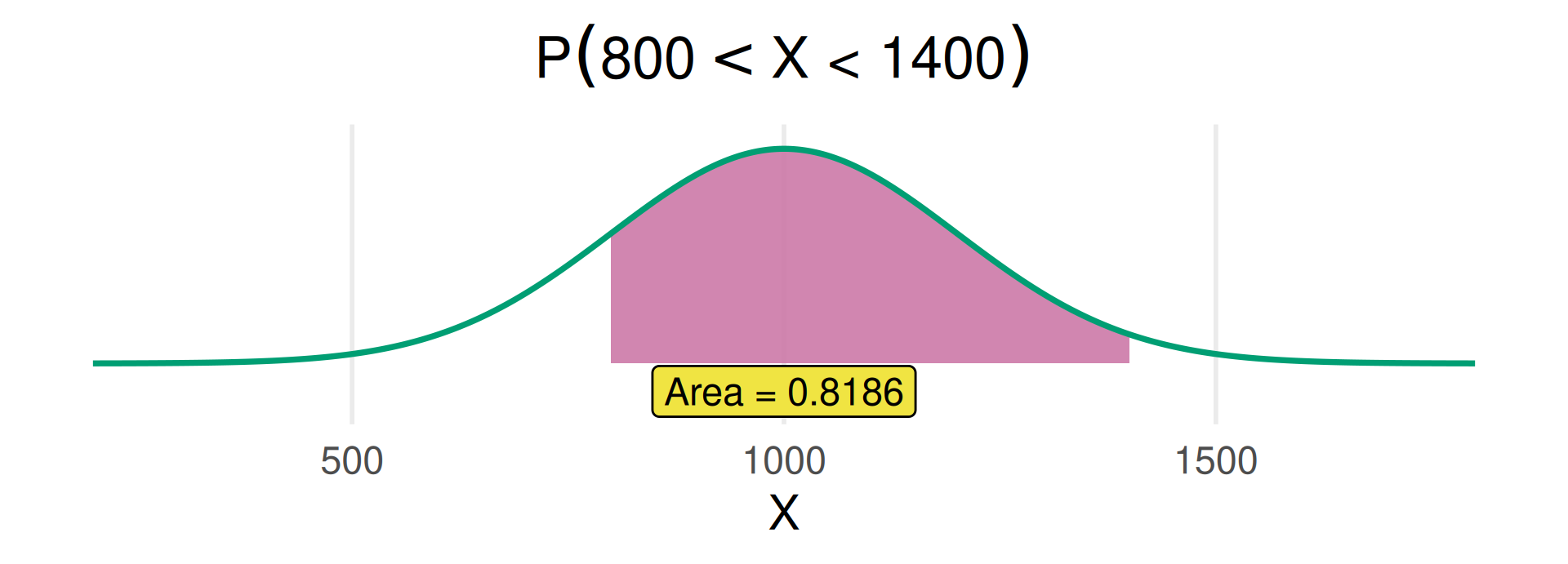
calc_prob_normal("x", mean =1000, sd =200, lower =800, upper =1400)
[1] 0.8185946
You can save it and use it with inline code:
prob_800_1400 <-calc_prob_normal("x", mean =1000, sd =200, lower =800, upper =1400)
About 82% of test takers scored between 800 and 1400.
Area to the left
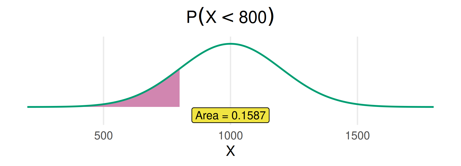
What is the probability that a randomly selected test taker scored below 800?
plot_normal("x", mean =1000, sd =200, upper =800)
calc_prob_normal("x", mean =1000, sd =200, upper =800)
[1] 0.1586553
Area to the right
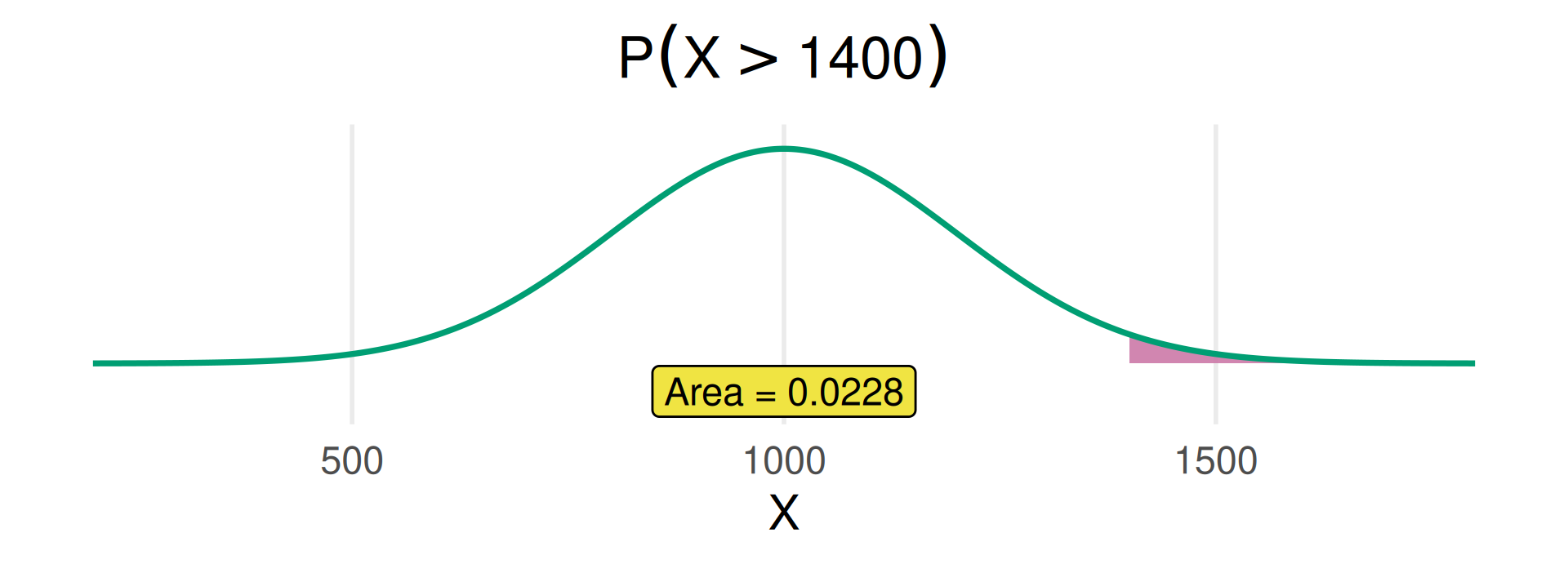
What is the probability that a randomly selected test taker scored above 1400?
plot_normal("x", mean =1000, sd =200, lower =1400)
calc_prob_normal("x", mean =1000, sd =200, lower =1400)
[1] 0.02275013
Area in between
What is the probability that a randomly selected test taker scored between 800 and 1400?
plot_normal("x", mean =1000, sd =200, lower =800, upper =1400)
The 68-95-99.7 rule
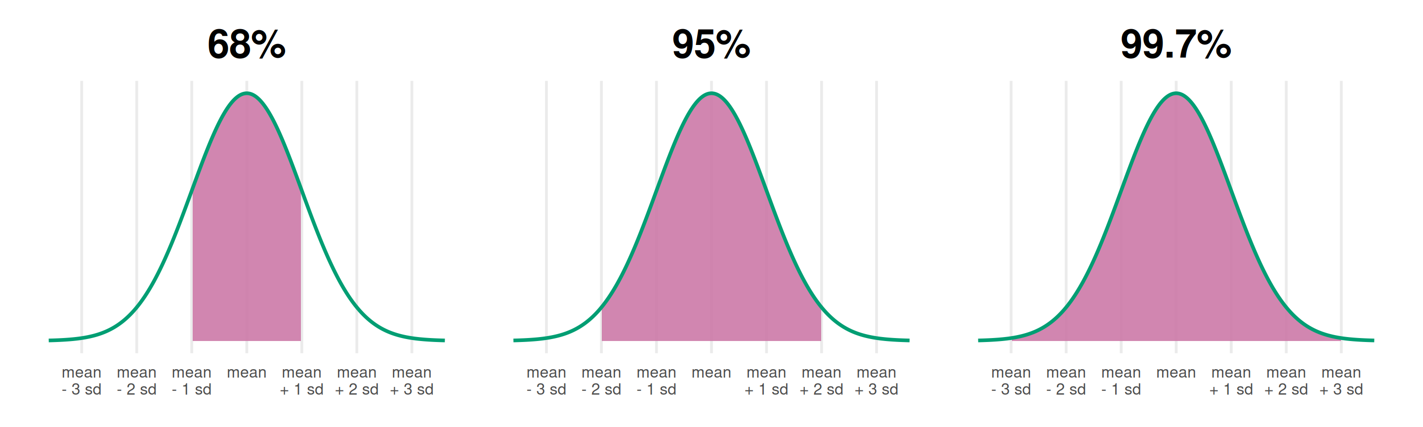
For any normal distribution, about 68% of the values are within 1 standard deviation of the mean, 95% within 2, and 99.7% within 3.
The 68-95-99.7 rule
Exercise
SAT total scores are approximately \(N(1000, 200^2)\). Without using R, find the approximate probability that a randomly selected test taker scored
between 800 and 1200.
between 600 and 1400.
above 1400.
above 1000.
Then check (a) and (c) with calc_prob_normal().
Match the picture
Exercise
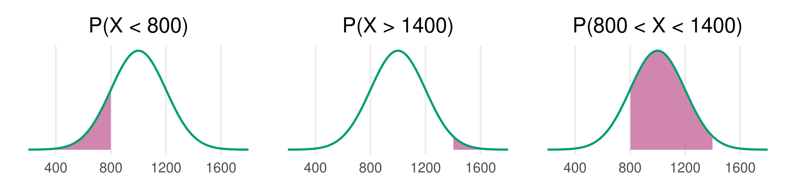
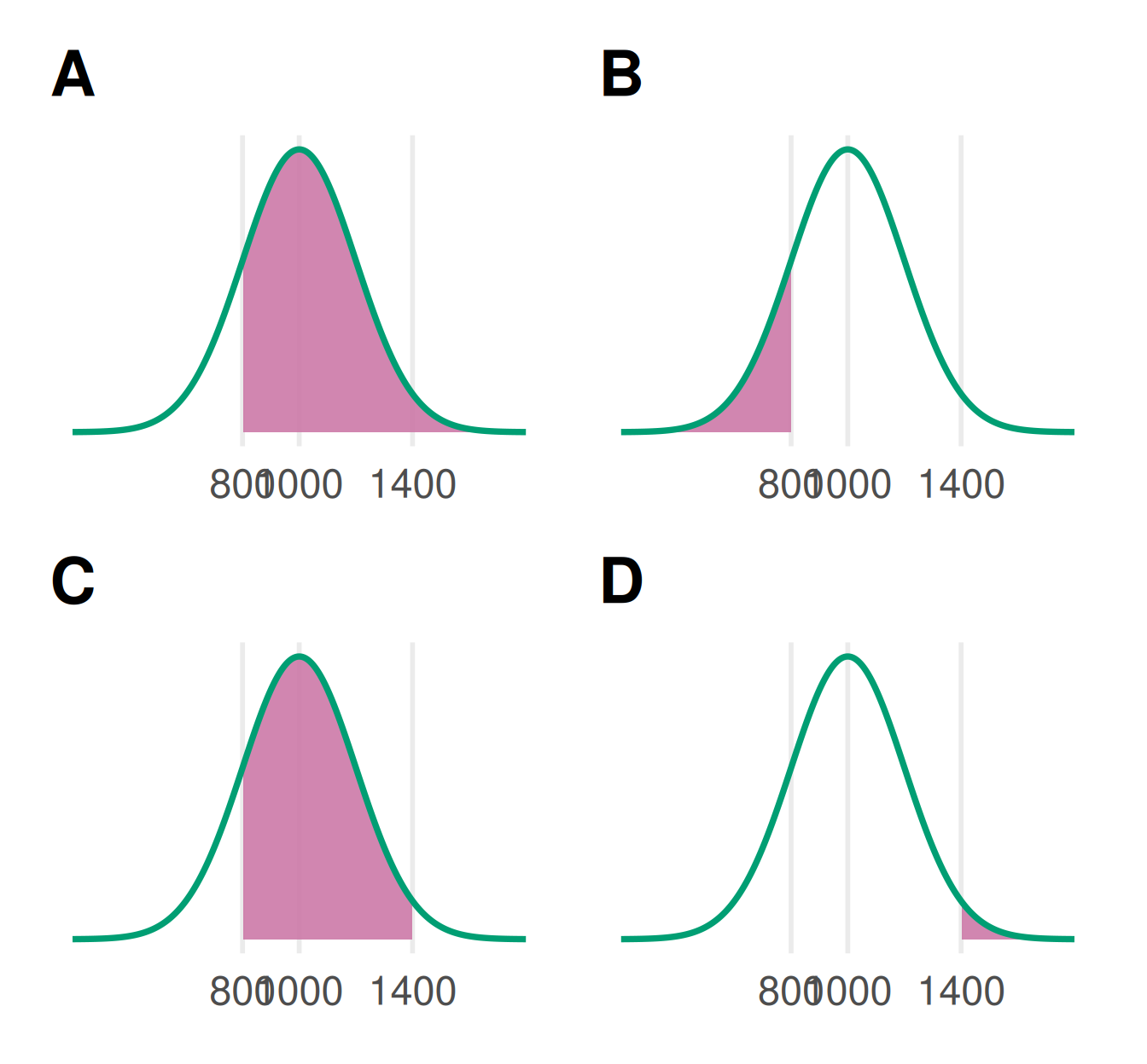
\(X \sim N(1000, 200^2)\). Match each picture to a probability.
\(P(X < 800)\)
\(P(X > 1400)\)
\(P(X > 800)\)
\(P(800 < X < 1400)\)
Then write the plot_normal() code for each.
Exactly 1200?
Discussion
\(X \sim N(1000, 200^2)\). According to this model, what is the probability that a randomly selected test taker scored exactly 1200? Not 1200.1, not 1199.99999, but exactly 1200.000000…
Exactly 1200? - answer
Answer: 0. The area of a single line under the curve is 0.
Just like the broken alarm last class: for a continuous random variable, we only ask about probabilities of intervals. This also means \(P(X < 1200) = P(X \le 1200)\).
Real SAT scores are reported in steps of 10, so some students do score exactly 1200. The normal distribution treats scores as continuous: it is a model.
Going backwards: find_normal_value()
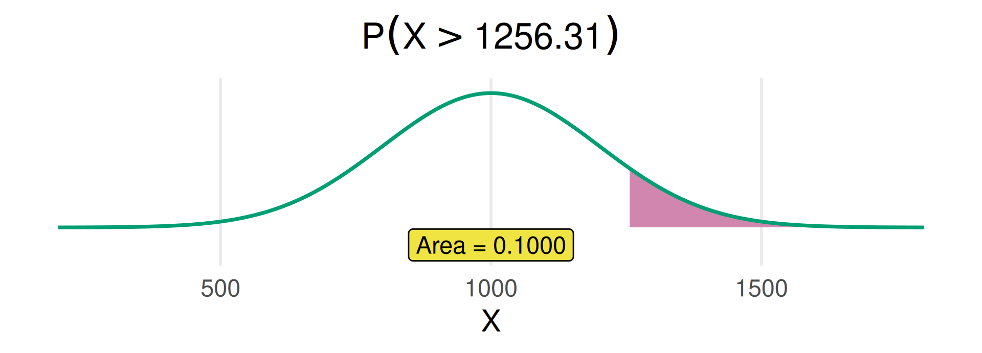
Sometimes we know the area and want the value. What total SAT score does a test taker need to be in the top 10%?
find_normal_value("x", mean =1000, sd =200, area =0.10, side ="above")
[1] 1256.31
Practice
Exercise
SAT Math scores are approximately \(N(500, 100^2)\).
What is the probability that a randomly selected test taker scored above 700 on SAT Math? Sketch the picture first, then use plot_normal() and calc_prob_normal().
What is the probability that a randomly selected test taker scored between 400 and 600?
What SAT Math score separates the lowest 25% of test takers from the rest?
z-scores
A z-score tells us how many standard deviations a value is away from the mean.
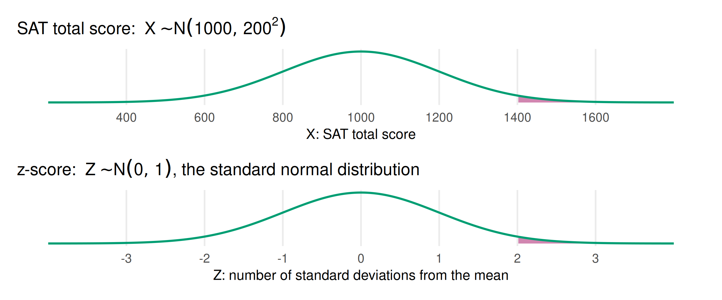
A total SAT score of 1400: \(z = \frac{1400 - 1000}{200} = 2\). The score is 2 standard deviations above the mean.
If \(X\) is normal, its z-score \(Z = \frac{X - \text{mean}}{\text{standard deviation}}\) follows \(N(0, 1)\), the standard normal distribution.
Normal vs. standard normal
A score of 1400 has \(z = \frac{1400 - 1000}{200} =\) 2. \(P(X > 1400) = P(Z > 2)\): converting to z-scores changes the numbers on the axis, not the shape or the areas.
z-scores
Exercise
SAT total scores are approximately \(N(1000, 200^2)\) and SAT Math scores are approximately \(N(500, 100^2)\).
Which is more unusual: a total SAT score of 1450 or an SAT Math score of 720?
Summary
A normal distribution is described by its mean and variance: \(N(\text{mean}, \text{variance})\). Check whether the second number is the standard deviation or the variance!
Probability = area under the curve: plot_normal() draws the area, calc_prob_normal() calculates it (value → area), and find_normal_value() goes from area → value.
The random variable can be a random observation (\(X\)) or a random population parameter that describes our uncertainty (\(\mu\), \(\pi\)). In a few weeks: random sample statistics (\(\bar{X}\), \(p\)).
A z-score is the number of standard deviations a value is from the mean. z-scores follow the standard normal distribution, \(N(0, 1)\).